Virus contig annotation pipeline
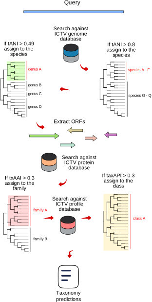
SKADI annotates viral contigs by sequentially comparing query sequences against nucleotide, protein, and profile databases using mmseqs2. The annotation process includes three stages.
Nucleotide database comparison
Query sequences are first compared to the nucleotide database using mmseqs_blastn. Optionally, users can switch to mmseqs_tblastx for higher sensitivity at the cost of longer run-times. skadi then tries to find the genome with the highest nucleotide similarity to the query seqeunce by approximating the ANIs between the query and genomes in the database. If the total ANI between the query and the targert is greater than 0.81, we assign the query to target’s species. Target’s genus is trnsfered to the query, if the tANI between them is between 0.49 and 0.81.
Here, total ANI (tANI) is defined as follows.
Let:
\( Q \) be an unknown virus contig that needs to be taxonomically annotated.
\( Nuc_{db} \) be a database of known virus genomes (here: ICTV genomes).
We search \( Q \) against \( Nuc_{db} \) to retrieve all matches for \( Q \) in \( Nuc_{db} \).
Let \( M_{db} \) be the list of genomic regions in \( TN_{db} \) that \( Q \) maps to.
\( M_n \subseteq M_{db} \) represents all regions similar to a target genome \(T_n\) with taxonomic assignment \( n \).
We calculate the total length of alignments to each taxonomic rank and the similarity of these alignments to \( C \) using:
where
Protein database comparison
For query sequences without significant nucleotide-level matches, open reading frames (ORFs) are predicted along the contig, and the resulting amino acid sequences are compared against the viral protein database. Based on these matches, we calculate the taxon Average Amino acid Identity (txAAI) between the query contig and each candidate taxon, and assign the query to the taxon with the highest txAAI.
This txAAI is conceptually different from a “total AAI” between two genomes or sequences, where AAI is computed directly between a single query genome and a single target genome by averaging the identities of their shared orthologs. In contrast, txAAI aggregates information across all matched proteins belonging to a taxonomic group (e.g. genus or family), potentially originating from multiple genomes within that group. As a result, txAAI reflects the overall similarity of the query contig to an entire taxon, rather than to any single reference genome, and is therefore better suited for taxonomic assignment in the presence of incomplete, fragmented, or diverse reference data.
Here, taxon AAI (txAAI) is defined as follows.
Extending the definitions above:
Let \( P_Q \) be the set of genes (ORFs) on \( Q \).
Let \( Prot_{db} \) be a database of viral proteins from ICTV genomes.
\( Prot_{db} \) is searched for matches to the ORFs found in \( Q \).
Let \( P_m \subseteq P_Q \) represent the subset of ORFs from \( Q \) that have significant matches in \( P_{db} \) to taxon \(n\).
\( I_{m_i} \) is the amino acid identity between the \( i \)-th matched ORF in \( P_m \) and its corresponding hit in \( P_{db} \).
Then the txAAI is:
where
Profile database comparison
Sequences that remain unannotated at the protein level are compared to a protein profile (HMM) database to provide taxonomic annotations.
Here, taxon API (txAPI) is calculated similarly to txAAI, except the target database is a protein profile (HMM) database instead of a protein sequence database.
Let:
\( H_{db} \) be the profile HMM database derived from ICTV viral protein families.
\( H_m \) represent the subset of ORFs from \( C \) that match profiles in \(H_{db}\).
\( S_{m_i} \) be the percent sequence identity (or bit-score-normalized identity, depending on implementation) between the \(i \)-th ORF and its matched profile.
Then:
where
Database Generation Pipeline
The skadi database generation pipeline automates the creation of comprehensive viral nucleotide, protein, and profile databases. The process includes the following steps:
1. ICTV metadata parsing and genome download
skadi parses the ICTV Metadata Resource and downloads all viral genomes and proteins from NCBI GenBank.
2. Custom taxonomy creation
A custom taxdump for the ICTV taxonomy is generated using taxonkit.
3. Nucleotide and protein database construction
Custom nucleotide and protein databases are created using mmseqs2, incorporating the ICTV-specific taxdump.
4. Protein clustering and profile database creation
Viral proteins are clustered, and these clusters are converted into a protein profile (HMM) database.